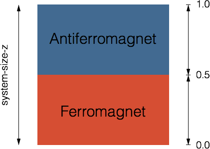
Vampire is capable of simulating up to one hundred different materials, in a wide variety of geometries such as core shell and multilayer systems. In this tutorial we set up a bilayer system consisting of a ferromagnet and antiferromagnet with different thicknesses. The multilayer system is created by specifying different magnetic materials with different heights in the material file, as shown in the schematic.
Since we are using the built-in geometric routines, we define the following parameters in the input file
dimensions:system-size-x=4 !nm
dimensions:system-size-y=4 !nm
dimensions:system-size-z=10 !nm
dimensions:unit-cell-size=3.5 !A
create:crystal-structure=sc
specifying the system dimensions, unit cell size and simple cubic crystal structure respectively. For continuous thin films it is also common to specify periodic boundary conditions in the film plane to remove any edge effects and reduction in the coordination number. With vampire this can easily be done by specifying
create:periodic-boundaries-x
create:periodic-boundaries-y
in the input file. While these parameters are suitable for simulating a generic thin film, the next step is to define two distinct materials for each layer. We do this by specifying that we are using two materials in the material file:
material:num-materials=2
In this example we will specify that the thickness of each layer makes up 50% of the z-height of the system. This is defined separately for each material using
material[1]:minimum-height=0.0
material[1]:maximum-height=0.5
material[2]:minimum-height=0.5
material[2]:maximum-height=1.0
With vampire the extent of the system along z is always defined as a fraction of the total system height, system-size-z. When dealing with effects for different film thicknesses, it is often easiest to specify a larger film thickness so that common increments in the film thickness are represented by simple fractions. For example, for a system 10 nm in height, fractions of 0.1 in the minimum and maximum height specify increments of 1 nm. Although this simplifies the system set up, if a large fraction of the defined system is empty (with no atoms present) this may prevent parallelisation of the system since the parallel decomposition always operates on the full system volume. Remedies for the parallelisation include defining exact fractional heights encompassing the whole volume or by using the replicated-data parallel decomposition. With each material having a specific minimum and maximum height this effectively defines the bilayer atomic system. The different materials can be identified visually by defining different atomic species, or elements, for each material and converting the atomic configuration output to a .xyz file for viewing in chemical structure viewers such as rasmol or jmol. There is a code in the vampire source code package (cfg2rasmol.cpp) which performs the conversion. The elements are defined as follows
material[1]:material-element=Ag
material[2]:material-element=Fe
and play no role in the simulation. However different elements appear with different colours on the molecular structure viewers allowing different materials to be easily identified. The final step is to define the magnetic parameters for each of the layers, such that one is a ferromagnet and the other is an antiferromagnet. This is done by specifying the exchange interactions between atoms of each material:
material[1]:exchange-matrix[1]=+11.2e-21
material[1]:exchange-matrix[2]=+11.2e-21
material[2]:exchange-matrix[1]=+11.2e-21
material[2]:exchange-matrix[2]=-11.2e-21
Here material 1 is a ferromagnet (Jij > 0) and material 2 is an antiferromagnet (Jij < 0). The exchange between the two materials (the interfacial exchange) is defined as a ferromagnetic interaction with the same strength as the bulk. Note that the interaction strength from material 1 to 2 must be the same as from material 2 to 1.
For an FM/AFM bilayer the ground state spin structure is important which depends on other parameters such as magnetic anisotropy. In order to obtain a physically realistic ground state the spins in the antiferromagnetic layer are given a random initial direction (equivalent to infinite temperature) while spins in the ferromagnetic layer are initialized in-plane along the x-direction. Adding an in-plane magnetocrystalline anisotropy and other parameters gives the final material file:
#---------------------------------------------------
# Number of Materials
#---------------------------------------------------
material:num-materials=2
#---------------------------------------------------
# Material 1 Ferromagnetic Layer
#---------------------------------------------------
material[1]:material-name=FM
material[1]:damping-constant=1.0
material[1]:exchange-matrix[1]=11.2e-21
material[1]:exchange-matrix[2]=11.2e-21
material[1]:atomic-spin-moment=2.0 !muB
material[1]:uniaxial-anisotropy-constant=-1.0e-24
material[1]:material-element=Ag
material[1]:minimum-height=0.0
material[1]:maximum-height=0.5
material[1]:initial-spin-direction=1,0,0
#---------------------------------------------------
# Material 2 Anti-ferromagnetic Layer
#---------------------------------------------------
material[2]:material-name=FM
material[2]:damping-constant=1.0
material[2]:exchange-matrix[1]=11.2e-21
material[2]:exchange-matrix[2]=-11.2e-21
material[2]:atomic-spin-moment=2.0 !muB
material[2]:uniaxial-anisotropy-constant=-1.0e-24
material[2]:material-element=Fe
material[2]:minimum-height=0.5
material[2]:maximum-height=1.0
material[2]:initial-spin-direction=random
The final step is to define the input file for the simulation. Here we define a simple time series as we simply need to integrate the system for a period of time to obtain the ground state configuration. Equilibrium properties are generally better simulated using Monte Carlo methods, and we also specify that the code should output the initial and final atomic spin configurations which can be post-processed to generate images of the spin structure.
#---------------------------------------------------
# System dimensions
#---------------------------------------------------
dimensions:system-size-x=4 !nm
dimensions:system-size-y=4 !nm
dimensions:system-size-z=10 !nm
dimensions:unit-cell-size=3.5 !A
#---------------------------------------------------
# Creation attributes
#---------------------------------------------------
create:crystal-structure=sc
create:periodic-boundaries-x
create:periodic-boundaries-y
#---------------------------------------------------
# Material files
#---------------------------------------------------
material:file=bilayer.mat
#---------------------------------------------------
# Simulation attributes
#---------------------------------------------------
sim:temperature=0.1
sim:total-time-steps=11000
sim:time-steps-increment=1000
sim:program=time-series
sim:integrator=monte-carlo
#---------------------------------------------------
# Data output
#---------------------------------------------------
output:time-steps
output:temperature
output:material-magnetisation
config:atoms
config:atoms-output-rate=10
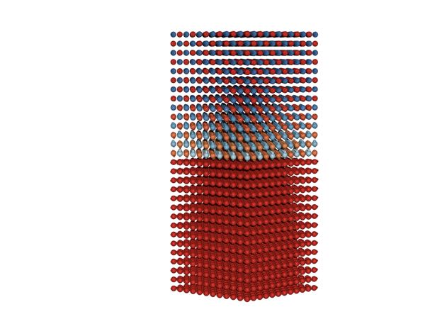
Running the simulation leads to the following ground state spin structure, showing the staggered spin state in the anti-ferromagnet and an in-plane magnetization for the ferromagnet. The same principles apply to generating multilayers, which can easily be done by specifying more materials with minima and maxima.
Copyright R F L Evans 2013-2018