Curie temperature simulation

The Curie temperature of a magnetic material is one of the most fundamental properties, as it is principally defined by the strength of the inter atomic exchange interaction. The exchange interaction is the strongest force in magnetism, as it determines the alignment of atomic spins, which makes a material ferromagnetic on the macroscopic scale. VAMPIRE contains a predefined function to calculate the Curie temperature of a material by performing a temperature sweep and calculating the average magnetisation, giving the classic M-T curve. This tutorial covers setting up the material and simulation parameters, running the simulation and analysing the results.

Step 1

The fist step is to define the material we wish to simulate. Due to the relative strength of the exchange interaction in most materials, we can safely ignore the other usual energy contributions, such as applied field and anisotropy, and so the spin Hamiltonian for our system reads:

H=J_ij ∑ S_i ⋅ S_j

where J_ij is the strength of the exchange interaction, S_i is the unit vector of the local spin moment i, and S_j is the unit vector of a neighbouring site j. In this Hamiltonian the exchange energy is calculated as a sum over nearest neighbours, as generally exchange is quite a short ranged effect. For our generic system, the exchange energy is isotropic (it doesn't vary with direction) and the same for all interactions, and so the exchange constant J_ij is taken outside the sum. For more complicated systems the exchange energy can be anisotropic and and be different for different interactions, in which case the exchange energy is interaction dependent and appears inside the sum. For ferromagnetic exchange, the sign of J_ij is positive.

The exchange constant is related to the Curie temperature T_c by the relation:

J_ij = 3k_BT_c / ε z

Where z is the number of interactions, Jij is the inter atomic exchange interaction, k_B is the Boltzmann constant and ε is a correction factor relating to spin wave stiffness [1]. For the 3D classical Heisenberg model ε is approximately 0.719 for a face-centred cubic system with 12 nearest neighbours. In this tutorial we will simulate a material with a Curie temperature of approximately 700K and with a simple cubic crystal structure, so applying this gives a round number value of J_ij = 6.72 x 10^-21 J/link.

Having defined the Hamiltonian we wish to use, we can now specify the material file:

#---------------------------------------------------
# Number of Materials
#---------------------------------------------------
material:num-materials=1
#---------------------------------------------------
# Material 1 Generic Ferromagnet
#---------------------------------------------------
material[1]:material-name=FM
material[1]:damping-constant=1.0
material[1]:exchange-matrix[1]=6.72e-21
material[1]:atomic-spin-moment=1.5 !muB
material[1]:uniaxial-anisotropy-constant=0.0

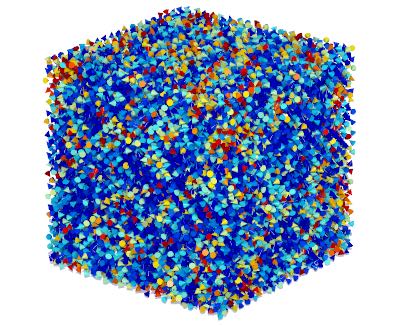
Here we define the exchange interaction and a material with zero anisotropy so we specifically set this to zero. For everything else the default parameters are fine, but we also define the atomic spin moment, the damping constant (used for dynamic simulations) and an identifying name for our material. The next step is to define the input file for the simulation. Since we want to approximate a bulk material, we define a reasonably sized system of (10 nm)³, which while not bulk is a sufficiently large number of spins that finite size effects are minimal.

Step 2

In order to remove surface effects we also define periodic boundary conditions in all three spatial dimensions:

create:periodic-boundaries-x
create:periodic-boundaries-y
create:periodic-boundaries-z

Step 3

Next we specify the simulation parameters we wish to use. The first of these is the integrator. Vampire has a choice of integrators, but the Monte Carlo method is excellent for the calculation of equilibrium properties, and so we choose this as follows:

sim:integrator = monte-carlo

To run the Curie temperature calculation we select the built in program as follows:

sim:program = curie-temperature

which performs a step-wise loop over temperature, performing equilibration and averaging steps and calculating the mean magnetisation before incrementing the temperature. The basic idea here is that when we calculate the Curie temperature we want the thermodynamic average of the magnetisation at that temperature. However, when experiencing a sudden drop in temperature the system takes a finite amount of time (or integration steps in the case of Monte Carlo integration) to reach thermal equilibrium. A typical time-dependent magnetisation caused by a stepwise increase in temperature is shown below.

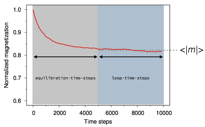
The magnetisation decreases exponentially toward a new average value. It is therefore important to make sure that thermal equilibrium is reached before taking an average of the magnetisation. In Vampire the curie temperature program includes both equilibration and averaging loops, which can be set using the sim:equilibration-time and sim:loop-time-steps variables respectively. Another point to note is that generally the time needed for equilibration is temperature dependent, and gets significantly longer around the Curie temperature, an effect known as critical slowing down. Generally 10,000 equilibration steps are sufficient for most systems, and so we can set the loop and equilibration times as follows:

sim:equilibration-time-steps = 10000
sim:loop-time-steps = 10000
sim:time-steps-increment = 1

Here we also set loop time to 10,000 steps to give a reasonable average. Increasing the number of averaging steps (set by sim:loop-time) will generally lead to smoother data. The time step increment determines the number of steps (or Monte Carlo moves) are made between taking statistical averages of the magnetization. Since we generally desire many samples, we explicity set this to 1 so that the magnetization is calculated after very complete Monte Carlo move and added to the average. The Curie temperature program also allows definition of minimum and maximum temperatures, as well as the temperature increment. Since we expect a Curie temperature of around 700K we will specify a minimum of 0K, maximum of 1000K, and increment of 25K as follows:

sim:minimum-temperature = 0
sim:maximum-temperature = 1000
sim:temperature-increment = 25

Step 4

Finally we specify the data output we want, this time simply the temperature and average magnetisation to the output file and screen as follows:

output:temperature
output:mean-magnetisation-length
screen:temperature
screen:mean-magnetisation-length

The complete input file can be downloaded here. Running the simulation and plotting the data gives the following result:

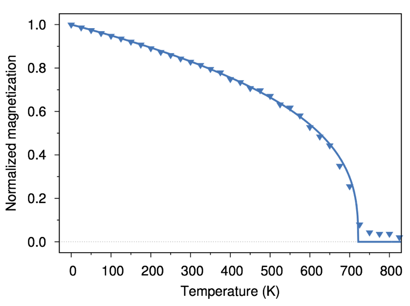
The Curie temperature is around 700K as we expected, and the shape of the curve is characteristic of the classical spin model. The analytic form of the normalised temperature dependent magnetisation for a generic ferromagnet is given by:

m(T) = (1 - T/T_c)^β

Fitting the data to the analytic form (shown by the line in the figure) shows excellent agreement with what we expect. Finally a small magnetic tail, where the magnetisation is not zero, is seen above the Curie point. This is a finite size effect, since due to the small size of the system there is a finite probability of a spontaneous instantaneous magnetisation, which leads to the visible tail.